Pressure projection methods

[LXX]

Hello, everyone. I’m a beginner in FreeFEM.

Currently, I’m attempting to decouple the velocity field and pressure field of the Navier-Stokes equations using the pressure projection method. In the first step, I aim to calculate the convergence order to validate the accuracy of my code. However, I’ve encountered some issues.

Here is my codetest_pressure_projection.edp (3.7 KB). I’m not sure whether it’s an issue with my understanding of the projection method or simply a coding problem.

The format I’m using is:

[fb77 (François Bouchut)]

Hello,
Your algorithm is correct (but you need to take care of the boundary condition on p^{n+1}, this is a sensitive point). You forgot to code the convection. Moreover your computation of right-hand side f was mistaken.
The way you evaluate the order of convergence is not good: you cannot evaluate the convergence in time by diminishing the timestep at fixed mesh. You need to reduce both simultaneously (I did not modify that).
Francois.
test_pressure_projection.edp (3.9 KB)

[LXX]

Thank you very much for responding to my questions.

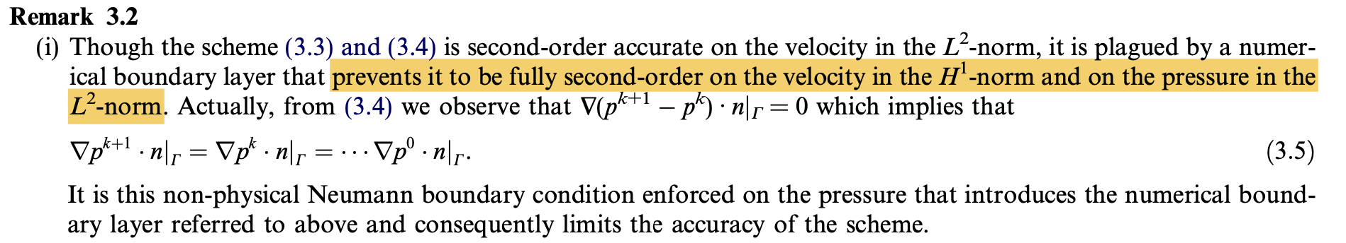
I looked up some references on the pressure projection method. In the second variational problem of updating pressure, the Neumann boundary condition of pressure is required. In practice, this condition is responsible for the errors this method shows close to the boundary of the domain since the real pressure (i.e., the pressure in the exact solution of the Navier-Stokes equations) does not satisfy such boundary conditions. But if the velocity can satisfy u·n=0 boundary condition, the Neumann boundary conditions of the pressure will naturally be obtained.

I see that what you added in the code is on(1,2,3,4,pnp1=pe(t))Dirichlet boundary condition. Is it correct?

Convergence order in L2 norm of u: 0, 0.158643, 1.05926, 0.962136, 0.74141, 0.496186. 
Convergence order in H1 norm of u: 0, 0.153184, 0.967829, 0.871569, 0.691116, 0.541268. 
convergence order in L2 norm of p: 0, 1.72902, -1.21749, 0.519209, 0.767257, 0.801716.

Is this the result of me running the code, or is it incorrect and is it caused by the above issue?

In addition, for the convection term, do I have to use convect? Can’t I define macro UgradV(ux,uy,vx,vy) [ux*dx(vx) + uy*dy(vx), ux*dx(vy) + uy*dy(vy)] // myself?

[fb77 (François Bouchut)]

I put Dirichelt BC on p with the exact solution on the boundary in order to be sure that you get the right solution. This is of course nor possible when you do not know the exact solution. Thus in general you need to do something else, and I am not at all expert on that (it seems that you know more than me on that).
For the convection you can do it also with UgradV implicitly, but for that you need enough viscosity for it to be stable.

[LXX]

Thank you very much for your reply. I have two more questions.

In 3D, the convection term is expressed as convect([u1,u2,u3],−dt,cold) ？

In addition to the convection, are there other expressions affected by physical parameters, such as the diffusion second-order curl term curl(curl B) and the convection first-order curl curl(B \times u)$ in the magnetic fluid equation? Can I define curl and cross product operators directly using macro?

macro curl(Bx,By,Bz) [dy(Bz)-dz(By), dz(Bx)-dx(Bz), dx(By)-dy(Bx)] //
macro crossProduct(ux,uy,uz,vx,vy,vz) [uy*vz-uz*vy, uz*vx-ux*vz, ux*vy-uy*vx] // 

[fb77 (François Bouchut)]

I have not tried convection in 3d, but your formula looks correct. Your macros are correct also, except that you must put some () for cross product:
macro crossProduct(ux,uy,uz,vx,vy,vz) [(uy)*(vz)-(uz)*(vy), (uz)*(vx)-(ux)*(vz), (ux)*(vy)-(uy)*(vx)] //
This is because macro performs a formal replacement with the arguments (the arguments have to be understood as strings, not as numbers).
In case the argument ux is “a+b” the macro without parenthese would produce terms
-a+b*vz and a+b*vy, missing parentheses!

[LXX]

Thank you ,Professor. I will correct the code.

[LXX]

Hello dear professor.
I looked up some more information about the pressure projection method. Now, regardless of the accuracy of this method, I want to add the following boundary conditions to the second step update pressure and the third step update speed, how do I enter the code?

The boundary condition of the pressure in the second step is derived from u·n = 0 ( or = ue·n )

Here’s my updated theoretical algorithm

[fb77 (François Bouchut)]

The equation you have to solve for p^{n+1} is a Laplace equation with non homogeneous Neumann boundary condition.
You can look at this post

Uzawa scheme for stokes bingham flow

In that paper the flow is taken incompressible, whereas in your code you use compressible. This is why the solution is different (but looks correct). You can modify easily your code to do the incompressible case, by using the extra variables p,q as solve bing([ux,uy,p],[vx,vy,q]) and adding -int2d(Th)(p*Divergence(vx, vy)+q*Divergence(ux, uy)) But then it happens that the scheme converges extremely slowly (you need thousands of iterations). In order to improve it you should use the Augmente…

From “We are thus led to the problem…”

[LXX]

Yes, professor. But why do not you enter f and g in this code? What is dyg2*(dy(ux) - dx(uy))? I want to know the weak form by which the code is written.

fespace Rh(Th, P2);
Rh dyg,dyg2;
solve streamlines (dyg, dyg2,solver=UMFPACK)
    = int2d(Th)(
          dx(dyg)*dx(dyg2)
        + dy(dyg)*dy(dyg2)
    )
    + int2d(Th)(
        - dyg2*(dy(ux) - dx(uy))
    )
    + int1d(Th)(
        - dyg2*(uy*N.x-ux*N.y)
    )
    + int1d(Th)(1e-8*dyg*dyg2)
    ;

[fb77 (François Bouchut)]

replace dy(ux) - dx(uy) by f
replace uyN.x-uxN.y by g

[LXX]

Okay, Professor. I understand what you mean.

Pressure projection method first step is to calculate \boldsymbol{\tilde{u}}, BC is \boldsymbol{\tilde{u}}|_{\partial\Omega} = 0, but for examples with analytical solutions \boldsymbol{u}_e, I think BC is \boldsymbol{\tilde{u}}|_{\partial\Omega} = \boldsymbol{u}_e. The third step is to calculate \boldsymbol{u}^{n+1}, which cannot use Dirichlet BC, so take \boldsymbol{u}^{n+1}\cdot\boldsymbol{n}|_{\partial\Omega} = 0(theoretical analysis), but For examples with analytical solutions, the boundary condition should be \boldsymbol{u}^{n+1}\cdot\boldsymbol{n}|_{\partial\Omega} = \boldsymbol{u}_e\cdot\boldsymbol{n}. Can I analyze it this way, professor?

So, I can get \nabla (p^{n+1} - p^n) \cdot \boldsymbol{n} = - \frac{\boldsymbol{u}^{n+1} -\boldsymbol{\tilde{u}}}{\Delta t}\cdot\boldsymbol{n} = 0. What should I enter for pressure BC:

solve pb4up(pnp1,pp) =...(omit this part)
+ int1d(Th)( (dx(pn)*N.x +  dy(pn)*N.y)*pp );

Is it right, professor?

[fb77 (François Bouchut)]

First remark, if the original problem you want to solve is u=0 on boundary, they you have that u_e=0 on boundary.
Then to solve the homogeneous Neumann BC for p^{n+1} or p^{n+1}-p^n, you use the formulation I sent with g=0. Thus the only int1d that remains is the one with 1e-8. You do not have to put the term dx(pn)*N.x + dy(pn)*N.y.

[LXX]

Okay, Professor. I understand what you mean.

The third step: update \boldsymbol{u}^{n+1} with \frac{\boldsymbol{u}^{n+1} -\boldsymbol{\tilde{u}}}{\Delta t} + \nabla p^{n+1} - \nabla p^n = 0. Should I use the variational problem and add the boundary condition \boldsymbol{u}^{n+1}\cdot\boldsymbol{n} = 0 or \boldsymbol{u}^{n+1}\cdot\boldsymbol{n} = \boldsymbol{u}_e\cdot\boldsymbol{n}, like this

solve pb4u(uxnp1, uynp1, vx, vy) 
    = int2d(Th)([uxnp1, uynp1]'*[vx, vy])
    - int2d(Th)([uxtilde, uytilde]'*[vx, vy] - dt(i)*grad(pnp1)'*[vx, vy] + dt(i)*grad(p0)'*[vx, vy])
    + int1d(Th,1,2,3,4)(1.e10*(uxnp1*N.x + uynp1*N.y)*(vx*N.x + vy*N.y) )
    - int1d(Th,1,2,3,4)(1.e10*(uxe(t)*N.x + uye(t)*N.y)*(vx*N.x + vy*N.y) );

This is my second step.

solve pb4p(pnp1, pp) = int2d(Th)(grad(pnp1)'*grad(pp)) - int2d(Th)(grad(p0)'*grad(pp) - div(uxtilde, uytilde)*pp/dt(i))
            + int1d(Th,1,2,3,4)(1e-8*pnp1*pp) ;

[fb77 (François Bouchut)]

The third step is an L^2 projection thus there is no boundary condition. You should not put any int1d.
Alternatively you can just set

uxnp1 = uxtilde - dt(i)*dx(pnp1)+ dt(i)*dx(p0);
uynp1 = uytilde - dt(i)*dy(pnp1)+ dt(i)*dy(p0);

This performs an interpolation instead of an L^2 projection.

[LXX]

Thank you very much, professor. I changed my code based on your guidance.
pressure_projection_BDF2.edp (6.0 KB)
This is the standard incremental pressure-projection method. The time format is BDF2, and the first step (n=0) is backward Euler. Linearized convection term:
n = 0, (\boldsymbol{u}^n\cdot\nabla)\boldsymbol{u}^n;
n >= 1, ((2*\boldsymbol{u}^n - \boldsymbol{u}^{n-1})\cdot\nabla)(2*\boldsymbol{u}^n - \boldsymbol{u}^{n-1}).

This is my output:

L2 norm error of u: 8.90828e-05, 5.76243e-05, 1.52496e-05, 3.91707e-06, 9.99719e-07, 2.78619e-07. 
H1 norm error of u: 0.00129628, 0.000582098, 0.000196062, 0.000120427, 0.00011179, 0.000111002. 
L2 norm error of p: 0.000535824, 0.000129077, 3.14533e-05, 8.38204e-06, 2.28884e-06, 6.33111e-07. 

Convergence order in L2 norm of u: 0, 0.62847, 1.9179, 1.96093, 1.97018, 1.84323. 
Convergence order in H1 norm of u: 0, 1.15505, 1.56995, 0.703146, 0.107374, 0.0102053. 
Convergence order in L2 norm of p: 0, 2.05353, 2.03695, 1.90784, 1.87268, 1.85409.

I really don’t understand why the H1 norm convergence order of velocity is so bad? I test time accuracy.

I refer to page 4 of this paper (taking Stokes equation as an example):
An overview of projection methods for incompressible flows.pdf (943.4 KB)

[emmawilson]

Could you please guide me why my post is hidden?

[LXX]

So sorry, I do not know why.

[fb77 (François Bouchut)]

What this paper says is also what I am thinking of: the Neumann boundary condition that is imposed on p is not necessarily satisfied by the exact solution. As a consequence it could be that the pressure well converges to the exact solution far from the boundary, but does not converge close to the boundary (probably within a length of the order of the mesh size). This is what is called a boundary layer. The consequence is that the convergence rate on the pressure could be lower than expected. The H1 norm of u has usually a behavior similar to that of the pressure.
I would expect a rate of 2 for L2u, and a rate of 1 (or lower) for H1u and L2p.
But this behavior is for when you refine also the mesh, not only the timestep as you do.

However this is not what you observe: you get a low rate for the H1 norm, and a surprisingly high rate for the pressure. This is a bit mysterious.
This could be due to the fact that you refine only in time, or to the BDF2 formulas that you apply to u but not to p. I don’t know. I am not sure also of the explicit treatment of the convection. You could try it implicit as for example
UgradV(uxbar, uybar, uxtilde, uytilde)

[fb77 (François Bouchut)]

Several comments:

1. After some tries, I find that taking the convection implicit is slightly better.

2. It is also slightly better in the step of computing utilde,
   to take the pressure guess as pbar= 2*pn-pnm1 instead of pn.
   Then it is also pbar in the step of computing pnp1 by the Laplace equation and

uxnp1 = uxtilde - dt(i)*dx(pnp1)+ dt(i)*dx(pbar);
uynp1 = uytilde - dt(i)*dy(pnp1)+ dt(i)*dy(pbar);

3. It seems that there is no boundary layer, since if we replace the Neumann boundary condition on p by Dirichlet p=p_exact, nothing changes.

4. The apparent lack of convergence in the H1 norm is due to the fixed mesh 100*100. Indeed an idea of the H1 error associated to the mesh can be obtained setting just after the definition of initial ux0,uy0

real errdiv0=sqrt(int2d(Th)(abs(dx(ux0)+dy(uy0))^2));
cout << "errdiv0 " << errdiv0 << endl;

The result is 1.4e-4.
This means that a typical H1 error induced by projection onto the finite element space is of this order. It follows that even for high order time integration and small timestep, the H1 norm cannot get below this value (without refining the mesh). This is the reason why once the H1 error attains this value, it will no longer decay.