Non homogeneous boundary and initial conditions

[quentin (H.Weng)]

Dear Chris:
I added a componet T for temperature and modified vR and vJ, but I am uncertain about the derivation of residual and Jacobian.
the equations are:

Here I put the code:

macro def(u)[u, u#y, u#T, u#p]//
macro grad(u) [dx(u),dy(u)]//EOM
macro dot(v, u) ( v * u + v#y * u#y + v#T * u#T ) //EOM
macro div(u) ( dx(u) + dy(u#y) ) // velocity divergence
macro ugradu(v, U, u) ( v * (U * dx(u) + U#y * dy(u)) + v#y * (U * dx(u#y) + U#y * dy(u#y)) ) // scaled convection term
macro visc(v, u) ( dx(v) * dx(u) + dy(v) * dy(u) + dx(v#y) * dx(u#y) + dy(v#y) * dy(u#y)) // EOM
varf vR(def(dub), def(v)) = int2d(Th)(ugradu(v, ub, ub) - div(v) * ubp + visc(v, ub) * nu - vp * div(ub)
                          + grad(ubT)' * [ub,uby] * vT+ Kappa *  grad(ubT)' * grad(vT)- ubT * vy) //newly added
                          + on(1,2,3,4, dub = ub, duby = uby) + on(1,dubT=ubT-1) + on(3,dubT=ubT);
varf vM(def(dub), def(v)) = int2d(Th)(dot(v, dub))
                          + on(1,2,3,4, dub = ub, duby = uby) + on(1,dubT=ubT-1) + on(3,dubT=ubT);
varf vJ(def(dub), def(v)) = int2d(Th)(sig * dot(v, dub) + ugradu(v, ub, dub) + ugradu(v, dub, ub) 
                          + Kappa *  grad(dubT)'* grad(vT)+  grad(dubT)'* [ub,uby] * vT	 - dubT * vy//newly added
                          - div(v) * dubp + visc(v, dub) * nu - vp * div(dub)+epsp * dubp * vp)
                          + on(1,2,3,4, dub = ub, duby = uby) + on(1,dubT=ubT-1) + on(3,dubT=ubT);

Is there anything wrong with my varfs? And how to add a disturbance to ub[] to induce the startup? I tried to add a disturbance to ub[] but failed.

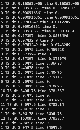
Also, I tried to run it to t=100, but stopped at step 962, what’s the problem? Should I adopt a finer mesh?
I monitored the temperature field, it looks reasonable.

[cmd (Chris)]

For one thing, you did not include the time derivative for temperature in your varf for vM() and vJ()…

[quentin (H.Weng)]

What does it mean? My understanding for it to be dubT*vT,
and I thought adding v#T * u#T to dot is enough, thus the dot(v,dub) is referring to (v*dub+vy*duby+vT*dubT). What the correct form should be?

[quentin (H.Weng)]

Note that the macro definition to dot has also been changed, maybe not need to add vT*dubT again.

[cmd (Chris)]

Oh sorry, I see. I’m not sure then. Are you using reasonable values for the parameters given your mesh resolution? Your solution looks a bit wild – there may be numerical issues. I would start with a case with high dissipation and move from there.

[quentin (H.Weng)]

Hi, Chris,
just as you said, I can add an additional routine to solve thermal field in the function, now the problem is how to exchange the messages between the two fields.
In each step of NSE solved in the TSSolve, how to import the velocity filed [ub,uby]? In my previous serial code, I use restrict to update the field like:

int[int] rest= restrict(VhF,VhT,myN2O);//F denotes fluid and T denotes thermal
uT[](rest)=uF[];

then the velocity computed can be used to compute the temperature.
In the decomposed mesh, and with PETSc, how to handle with the two fields? My raw idea is to restrict between VhTglobal and VhFglobal, and in each step, reduce the local solution to global, then copy the solution from one to the other, and finally go from global to local.

Moreover, maybe brackets needed to separate macros like def(u), createMat for the two fields.

Could you give me some advice?

[cmd (Chris)]

You should be able to do restrictions just like you did in your serial code.

Yes, you can use brackets to separate macros as you suggest. For example:

macro createMat1(th,A,P){
    NewMacro def(u)[ub, uby, ubT] EndMacro
    NewMacro init(i)[i,i,i] EndMacro
    createMat(th,A,P)
} // EOM
macro createMat2(th,A,P){
    NewMacro def(u)[ub, uby] EndMacro
    NewMacro init(i)[i, i] EndMacro
    createMat(th,A,P)
} // EOM

[quentin (H.Weng)]

Hi, Chris.
How to restrict between the two global meshs but without decomposition? I mean, it seems that restrict must after a buildDmesh or createMat, it will decompose the mesh. In my serial code, I use -n 1 so there no such problem.

[cmd (Chris)]

Sorry – I thought you were restricting two fespaces on the same mesh. For two different meshes (with two different decompositions), I think you will have to do what you originally proposed:

@quentin

reduce the local solution to global, then copy the solution from one to the other, and finally go from global to local.

[quentin (H.Weng)]

I found a example using VecInterpolate, or transferto copy variables to another mesh.

Copy variables between different meshes with PETSc

Dear Tak, You can use the newly implemented routine transfer to help you go between one distributed solution to another. If you want the transfer PETSc Mat, you can use the transferMat function, see this new example PtAP-2d-PETSc.edp. Here is the function used in your code, and the resulting screenshots. load "PETSc" macro dimension()2// EOM include "macro_ddm.idp" meshN Sh1=square(30,30,[x,y]); meshN Sh2=square(50,50,[x,y]); buildDmesh(Sh1) buildDmesh(Sh2) fespace Ph1(Sh1, P2); Ph1 u=sin…

I’ll try this approach, it looks more convenient than restrictions.

[cmd (Chris)]

Nice find. Indeed, that looks best.

[quentin (H.Weng)]

After several trials I recognised that transfer is not for meshes in different domain, but for a coarse mesh and its refinement.
Finally the solution is using trunc to get a n2o array for restrict. The mesh region is defined in advance hence the fluid domain can be derived form the whole mesh(the thermal domain).

[quentin (H.Weng)]

Hi, Chris,@cmd
I added another TSSolve in the funcM to compute T, it will perform after each step of NSE but use value of previous step.
Is -ts_type the only thing to change when turning to other implicit schemes? Should I change vJ, vR or funcJ, funcF ?
The example advection-TS-2d-PETSc.edp introduces a new function funcExplicit for the explicit scheme:

func real[int] funcExplicit(real t, real[int]& in) {
    real[int] temp(in.n), out(in.n);
    MatMult(dK, in, temp);
    temp *= -1;
    KSPSolve(dM, temp, out);
    return out;
}

I am not sure how to write it in my code because the example adopts default tgv, and it uses

func int funcJ(real t, real[int]& in, real[int]& inT, real a) {
    if(abs(a - shift) > 1.0e-10) {
        matrix B = a * M + K;
        dT = B;
        shift = a;
    }
    return 0;
}

to update the Jacobian.
This question is out of an abnormal large time step on the beginning, the time steps will grow tenfold! So I want to change the time scheme.

[cmd (Chris)]

If you’re using a fully implicit scheme then you don’t need an explicit part.

See the PETSc manual for complete list of options for TSSolve.

If you want to turn off adaptive time stepping use
-ts_adapt_type none

[quentin (H.Weng)]

Sorry for another bother, I have a little problem: the velocity is exchanged in funcJ and funcF, when I do uglobal[](restriction)=ulocal[] and mpiAllReduce in funcM, the overlapping part will count more than 1 time.
Should I use a new FEfunction to store the unexchanged value?

[cmd (Chris)]

use

real[int] temp;
ChangeNumbering(J, ulocal[], temp); //assuming J is your Mat
ChangeNumbering(J, ulocal[], temp, inverse = true);

[quentin (H.Weng)]

@cmd

a better approach is to introduce a scalar Lagrange multiplier to constrain the average pressure to a fixed value. This requires you to augment the Jacobian matrix with a single row and column describing the constraint.

Hi Chris,
Thanks for your help, I can run my simulation in parallel now. On the whole, the solution is plausible, but there remained some problems which may come from the conservation of mass. So I hope for a better approach.

Could you please elaborate the Lagrange multiplier? Sorry that I know little about it.

If my understanding is correct, the Jacobian J is replaced by [[J,b],[b',0]], and bgets from
varf vL(def(dub),def(v)) =int2d(Th)(vp);,right?

And, how to modify the code to cope with the augmented matrix? The size of PETSc numbering is larger than FE function array, I tried to use

real[int] tmp=in(0:in.n-2);
    ChangeNumbering(TS, ub[], tmp, inverse = true, exchange = true);

in funcs but end with error.

[cmd (Chris)]

You can see a full example here

You can also find some simpler MWEs in the examples/hpddm folder of the FreeFem package.

[quentin (H.Weng)]

Thanks a lot, I will check it out.

[quentin (H.Weng)]

Hi Chris,
I met some problems with the DNS.

1. I use -ts_type bdf -ts_bdf_order 3 and set -ts_dt 0.05, -ts_adapt_type none, the time step is fixed in the beginning, but after a while, the step changed to a quarter of the previous one, and finally it was stuck.
   Here’s the error message from console, you can see in step 725, dt became 0.0125, and finally it became about 7*10^-10!
   
   
   
   

   
   
   I found a larger dt will not bring such behaviour. If I use -ts_dt 0.25, then the step won’t change.

2. I tried to enlarge the scale of the problem to compute the flow under larger parameters. I allocate processes proportional to the DoFs, but it became slow obviously. The local submeshes is almost the same scale, why the larger global mesh given a worse performance?

Could you give me some advice?