Question about movemesh in parallel

[zxss]

Dear all,

I am implementing Navier Stokes equations with moving boundary using ALE method. I want to parallelize it. Firstly, I directly movemesh in parallel without ‘move the global mesh in a single processor‘, and the result seems normal.

parallel_moving_boundary.edp (3.0 KB)

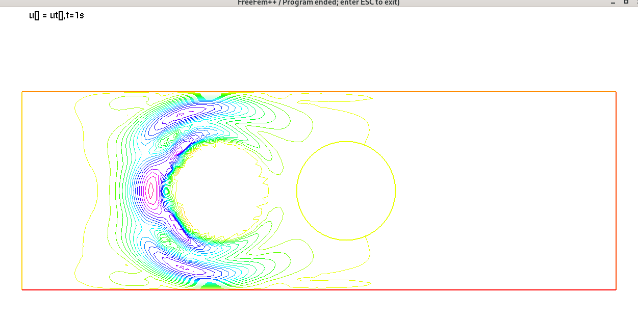
However, when I you try to centralize mesh velocity function, move global mesh in a single process, and re-decompose, something strange happened. The rigid cylinder deforms

The changed code is

withRediscompose.edp (4.4 KB)

I suspect that there is something wrong of my changed code about redecompose part. Because when I choose 1 processor, the rigid circle still deforms.

[prj]

If the code does not produce the desired results even with a single process, then that needs to be fixed first and foremost.

[zxss]

Sorry for my late reply. I am still debugging. And I find something intersting when I use composite fespace in my sequential code

Composite_fespace.edp (2.1 KB)

That is, when I solve the linear equation, if I make the arrays of two composite function equal

Rh [ut, vt, pt]; // intermediate function
ut[]=A^-1 * rhs;
u[] = ut[];

and when I do interpolation

Rh [ut, vt, pt]; // intermediate function
ut[]=A^-1 * rhs;
[u, v, p]=[ut, vt, pt]; 

these two results are different. And the latter is the same with using single fespace function.

single_fespace.edp (2.0 KB)

My question is what cause such a big difference with changing just one line from

u[] = ut[]; 

to

[u, v, p]=[ut, vt, pt]; 

Is it becuase the different ordering or something else?

[prj]

The figures you are plotting are not the ones from the .edp (which have no title). I don’t see a difference between both figures when I run your .edp.

[zxss]

Sorry, this time…

These two codes are the same except line 53, 54

[u, v, p]=[ut, vt, pt];

//u = ut;

Interpolation.edp (2.1 KB)

Array.edp (2.1 KB)

And the results are

[prj]

If you cout the solution, you’ll see they are the same, there is an issue with the plotting though, not really sure what’s going on.

[zxss]

Thanks for your prompt reply, I try to cout u, v and uu, at the end

with

cout<<u<<endl; cout<<v<<endl; cout<<uu<<endl;

and find that u and v are the same from both codes, uu is different.

Maybe there exists something wrong from this line

uu=sqrt(u^2+v^2);

where u,v are function from composite fespace Rh [u,v,p]

[zxss]

Dear professor, I have a further question, now I upgrade my sequential code into parallel code,

sequential.edp (2.1 KB)

parallel.edp (2.8 KB)

then I run them with FreeFem++ and ff-mpirun -n 1 (which is also sequential since only one processor is uses)respectively.

I find there exists a little bi difference from the plots of uu = sqrt(u^2+v^2);

the up is from sequential code and the bottom is from parallel code. I find the maxium values are different and the up looks smoother.

Is it because of different solvers? For sequential code, I choose

set(A,solver=GMRES);
set(Ae,solver=GMRES);

while for the parallel code, from -ksp_solve, I use ‘gmres’ with ‘lu’ for preconditioner.

I am not sure which one is more accurate.

[prj]

Switch from plotD to plot (or plotMPI) and you should get the same output (plotD only plots P_1 functions).

[zxss]

Many thinks, I got the same plots with

macro def(u)u// EOM

plotMPI(Thf, uu, P2, def, real, cmm = "magnitude of velocity");

Although I don’t know why a macro needs to be defined here…

[zxss]

Dear, professor,

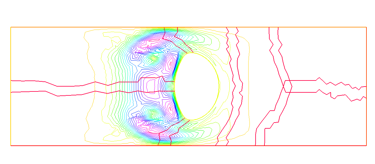
I want to do some numerical experiments to show the error when I directly use ‘movemesh‘ in parallel, and from the results, I find in this case, ‘movemesh‘ works well using 50 processors(maybe just a coincidence). The codes are

sequential.edp (2.1 KB)

parallel.edp (3.2 KB)

where the solvers are UMFPACK in sequential code and GMRES with LU (preconditioner)in parallel code. First of all, I got three plots using

FreeFem++ sequential.edp -wg -v 0

ff-mpirun -n 1 parallel.edp -wg -v 0

ff-mpirun -n 50 parallel.edp -wg -v 0

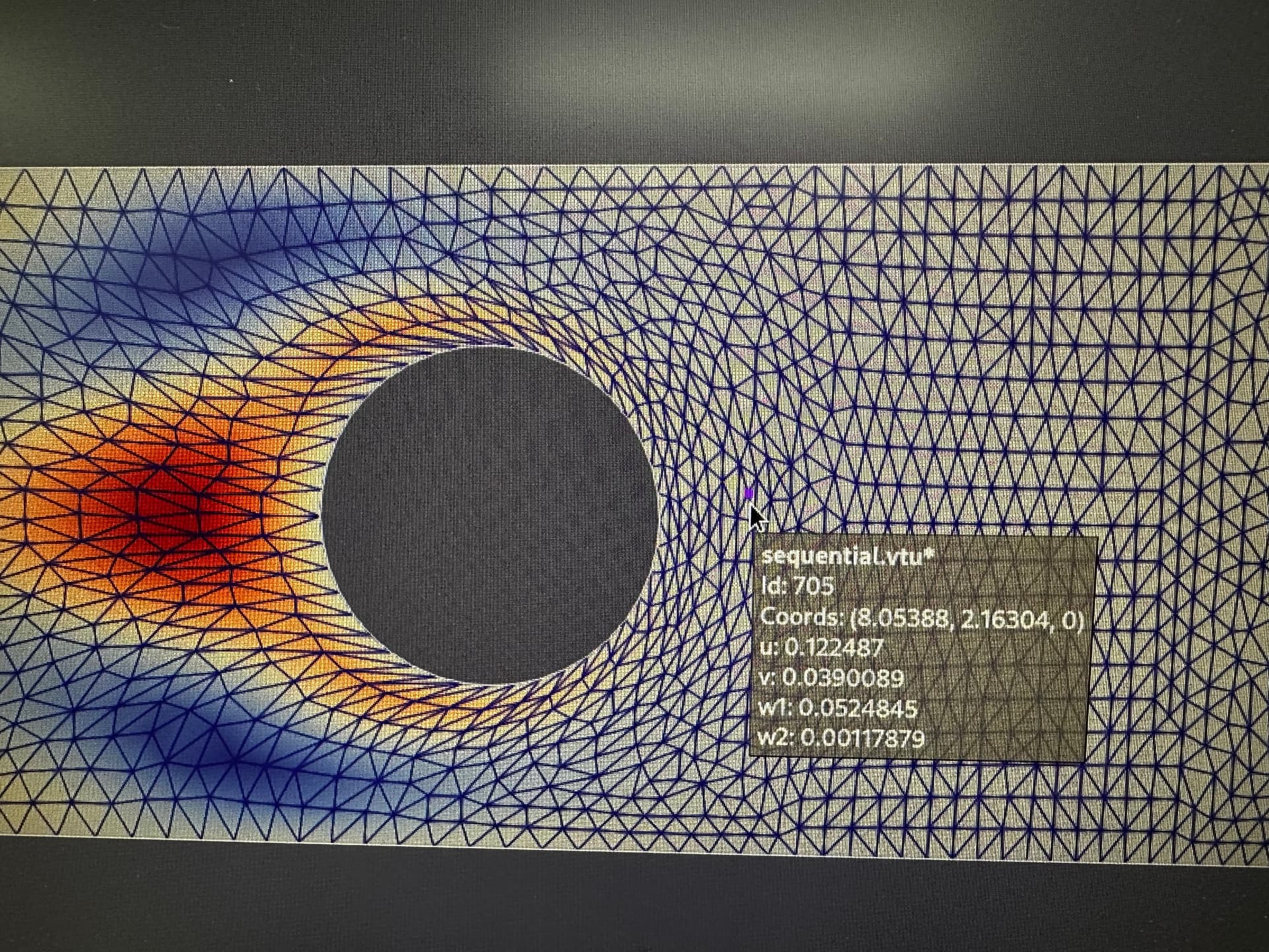
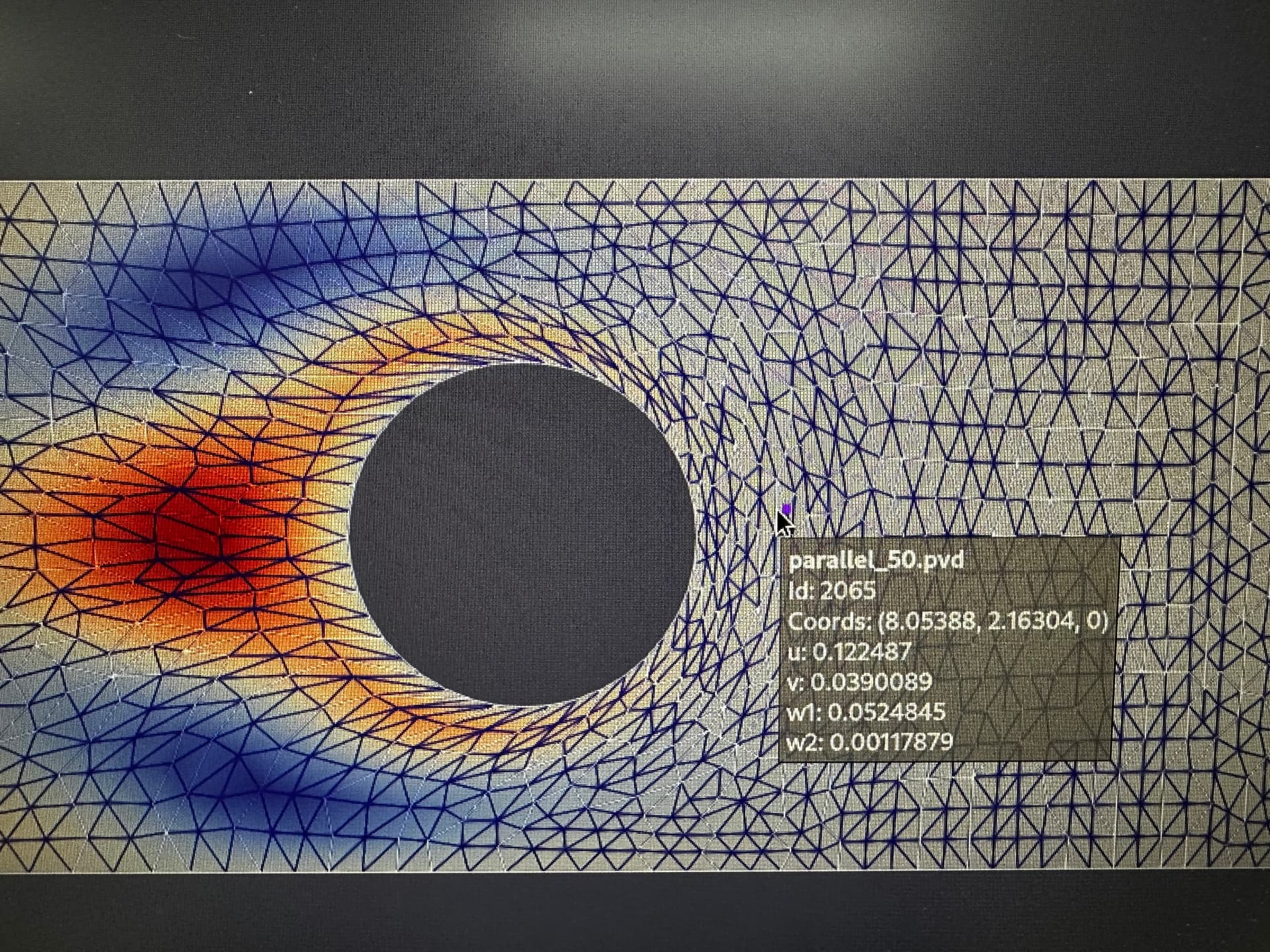
respectively (in order to magnify the error, under the assumption that more subdomains, more error, I choose 50 processors as comparison). From these three plots, they share the same maximum and minimum values. Since it’s just qualitative comparison. I try to do some quantitative comparisons in Paraview with .vtu files generated using ‘savevtk’ command.

for the sake of simplicity, here I only show one node of the last vtu/pvd file.

They share the same values of ‘u v w1 w2‘, and the only difference is the node index of 50 processors is different from others.

I want to figure out more details of

x=A^-1 * b;

where A is the distributed matrix. I want to talk about my understanding(maybe not correct), I use 2 processors and P1 element as an example

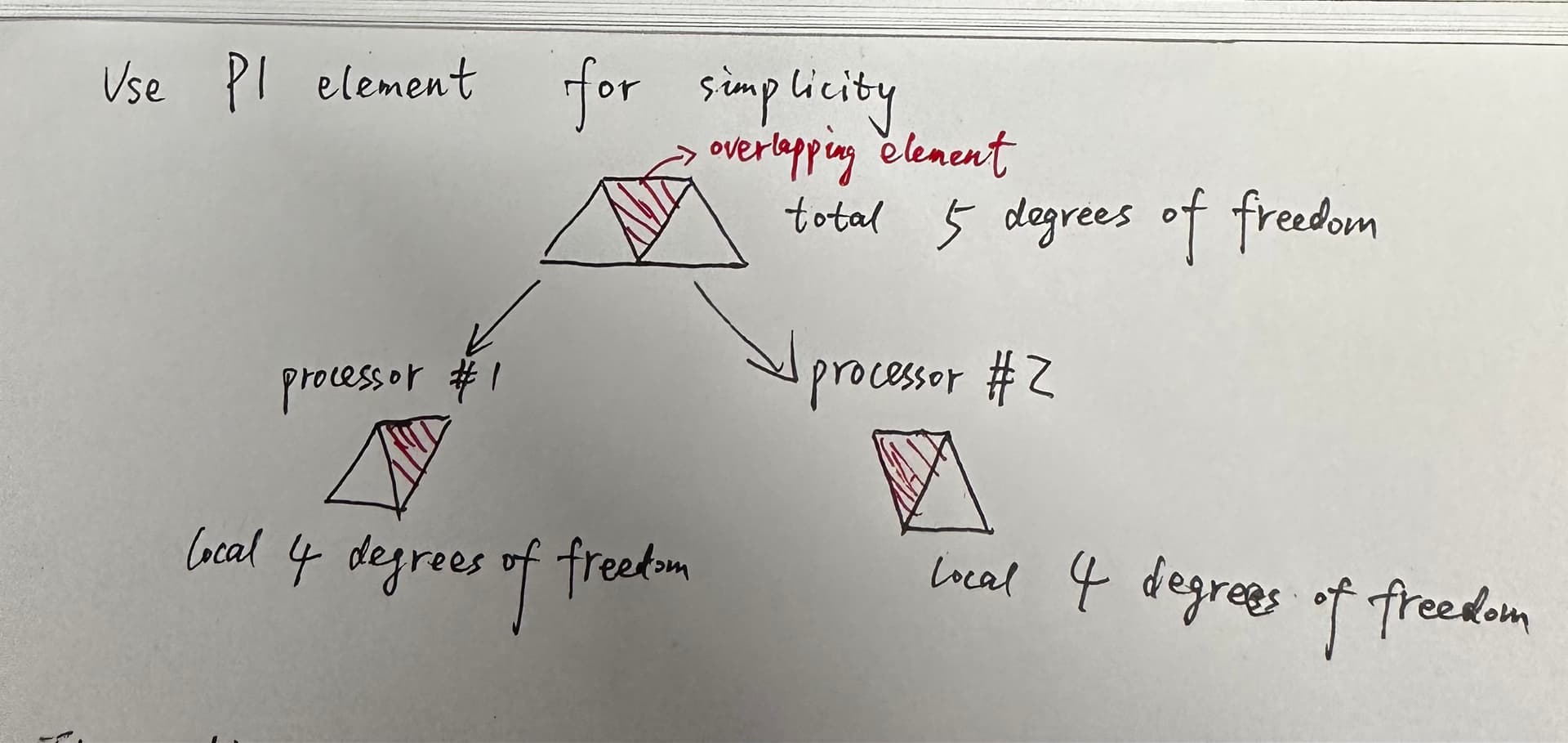
Since the ghost element actually belongs to one processor(here I assume it belongs to processor # 1), the distributed matrix A is a 5*5 matrix, after solving the linear system. The values of ghost element in processor # 2 are unknown. Are they given randomly?

[prj]

Of course they are not given randomly. Ghost values are consistent among processes after operations such as matrix-vector product and solution of linear systems.

[zxss]

Cool, then it can be explained why movemesh works well in this case,

because in

Thf = movemesh(Thf, [x+w1*dt, y+w2*dt]);

w1,w2 are mesh velocity function solved by an pseudo-elastic equation

varf elastic([w1,w2],[w1h,w2h])= int2d(Thf)(

trace(DD(w1,w2)\*DD(w1h,w2h)') + 10\*div(w1,w2)\*div(w1h,w2h) )

+ on(5,w1=4*sin(pi*t),w2=0)+on(1,3,w2=0)+ on(2,4,w1=0);

they are consistent over ghost elements.